Thermocouple Temperature Measurement
NOTE: Please keep in mind that endless white papers and
pages of text can be written on temperature. I have no intention of going to
deep into every aspect of temperature and temperature measurement.
Introduction:
The purpose
and scope of this blog is to create an open look at temperature and
temperature measurement. What I hope to accomplish is a broad overview of
the more common methods of temperature measurement and uncertainties of the
measurement process. I hope to focus on one of the most common temperature
sensor types, the Thermocouple. The primary focus will be placed on the
tried and true thermocouple, likely the longest living temperature sensor
and among the most common. We will look at thermocouple placement,
thermocouple signal conditioning and considerations in choosing a
thermocouple type for a specific application.
History:
While not
quite the accurate temperature measurement we have today the actual concept
goes back to around the year 1592.
Galileo is actually credited with the earliest methods of temperature
measurement. The following is taken from Agilent Technologies Application
Note 290:
“In an open container filled with colored alcohol, he suspended a long
narrow throated glass tube, at the upper end of which was a hollow sphere.
When heated, the air in the sphere expanded and bubbled through the liquid.
Cooling the sphere caused the liquid to move up the tube. Fluctuations in
the temperature of the sphere could then be observed by noting the position
of the liquid inside the tube. This “upside-down” thermometer was a poor
indicator since the level changed with barometric pressure and the tube had
no scale. Vast improvements were made in temperature measurement accuracy
with the development of the Florentine thermometer, which incorporated
sealed construction and a graduated scale”.
For all intensive purposes that was the first liquid in glass thermometer
used for temperature measurement. I only mention this because for those with
children seeking a good science fair project the evolution of temperature
measurement makes for an interesting project. Some off the shelf isopropanol
alcohol and some food coloring with tygon tubing and a basic crude liquid
thermometer can be built. Over the years scales were developed. One scale,
however, wasn’t universally recognized until the early 1700’s when Gabriel
Fahrenheit, a Dutch instrument maker, produced accurate and repeatable
mercury thermometers. Mercury in glass thermometers served hundreds of years
as precision laboratory grade thermometers for accurate temperature
measurement and comparison purposes.
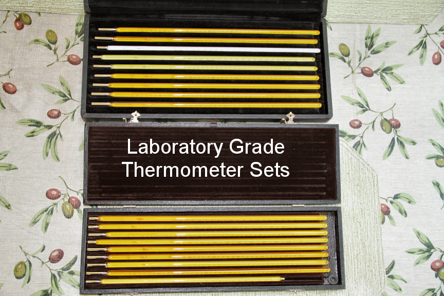
Laboratory Grade Thermometer Sets
Definitions and Terminology:
Throughout
this blog we will be using some terms and definitions. To avoid confusion we
should clarify those terms now as they apply to this blog. I will try to
make the definitions short and sweet.
1.
Accuracy:
Unbiased precision with a high measure of repeatability..
2.
Calibration:
That which is a comparison of a known to an unknown value of measurement.
3.
Resolution:
The ability to read an
instrument or of the instrument to be read.
The Thermocouple:
When two
wires made of dissimilar metals or alloys are joined at both ends and one of
the ends is heated an electric current flows in the loop. This becomes a
thermoelectric circuit. Thomas Seebeck made this discovery around the year
1821 and it is known as The Seebeck Effect. Note that there is a current
flow in the following thermoelectric circuit.
Figure 1
All dissimilar metals exhibit this effect. However,
certain combinations when paired have become the combinations used for our
more common thermocouples. They and their respective milli-volt outputs may
be seen in the following illustration.
Figure 2
Enter the different types of thermocouples. The chart in
figure 2 shows the six most common metal combinations used for making
thermocouples. They are given Type Designations and the chart shows Type E,
J, T, K, R and S type thermocouples. The chart also plots the milli-volt
output against temperature. This type of data becomes very important in
helping a designer choose a thermocouple for a desired range of temperature
and output. Thermocouple types are chosen based on their intended
application! Let’s take a look at the actual alloys that comprise these
thermocouple types.
Type Metals:
E
Chromel
(+) vs. Constantan (-)
J Iron (+) vs. Constantan (-)
K Chromel (+) vs. Alumel (-)
R Platinum (+) vs. Platinum 13%
Rhodium (-)
S Platinum (+) vs. Platinum 10%
Rhodium (-)
T
Copper (+) vs. Constantan (-)
While the milli-volt output of thermocouples is non-linear in nature they do
have somewhat linear regions. This is another important factor in choosing a
thermocouple for a desired application. Let’s take a look at the linearity
curves shown in figure 3.
Figure 3
We notice that the slope of the type K thermocouple approaches a constant
over a temperature range from 0°C to 1000°C. Consequently, the type K can be
used with a multiplying voltmeter and an external ice point reference to
obtain a moderately accurate direct readout of temperature. That is, the
temperature display involves only a scale factor. While that looks good it
is not quite true. Yes, a type K thermocouple does have a nice linear range
it is far from flat. Thermocouple outputs, all thermocouple outputs are a
non linear voltage out function. Therefore linearization is always necessary
for a thermocouple if we expect to achieve any accuracy.
CJC (Cold Junction Compensation):
Earlier we mentioned and explained the Seebeck Effect and used a small
illustration to show it. Let’s take a look at connecting a thermocouple to a
voltmeter (figure 4) and see what really happens. We know a junction of two
dissimilar alloys or metals form a thermoelectric junction so let’s see what
is really involved with measuring a thermocouple output accurately. We will
be using a Type K thermocouple for our example but the same rules would
apply for any thermocouple.
Figure 4
Measuring the output milli-volts of a thermocouple is not as easy or simple
as it may seem. Look at figure 4 and we notice junctions 2 and 3. We created
those junctions when we connected our copper DMM leads to the actual
thermocouple alloy leads. The actual hot junction is the thermocouple; the
cold junction is where the thermocouple alloys mate with or connect to the
DMM leads.
Accurate thermocouple
temperature measurement requires a stable reference junction. It is common
practice to create a transition reference junction by attaching a copper
lead wire to each thermocouple leg. When the transition reference junction
is held at the ice point 0°C (32°F) the output of the thermocouple appearing
across the copper leads attached to the readout instrument is stable and
predictable. This is only provided for reference as devices as seen in
Figure 5 would not be all that common outside a lab environment where
thermocouples were actually calibrated. They would represent Junction 2 and
Junction 3 in figure 4.
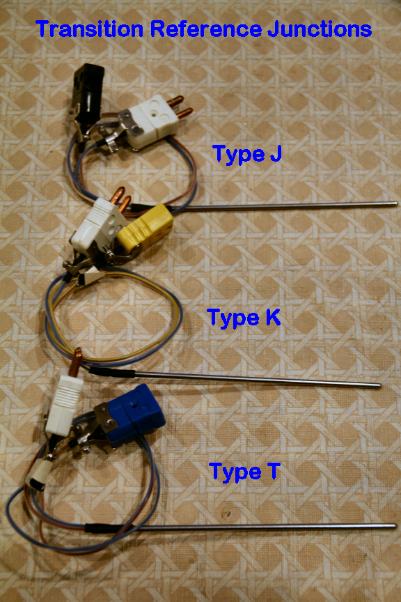
Figure 5
Let’s take a
look at an actual photograph of what Figure 4 would look like. The
thermocouple is a generic Type K thermocouple, laying on a table at room
temperature. The DMM is using copper clips connected directly to the
thermocouple.
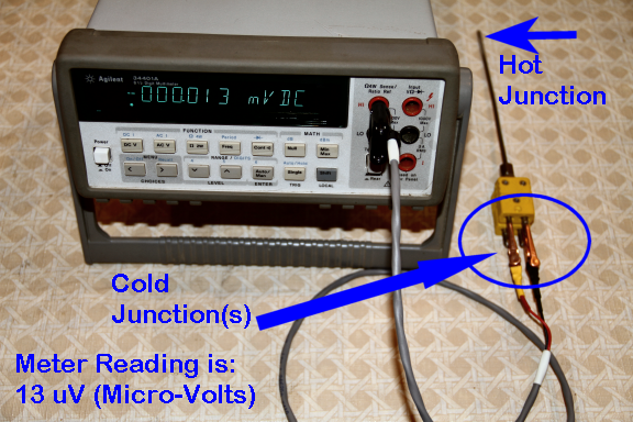
Figure 6
The ambient room
temperature is about 67 degrees F (19.44 C) and I know this to be true
because I measured it with precision mercury in glass calibrated laboratory
grade thermometer. Figures 7 & 8 illustrate how this is done. The
thermometer bulb is placed directly on the junction and allowed to
stabilize. This is shown in Figure 7 and the temperature is shown in Figure
8.
If I look up
a Type K temperature table I see that for my temperature I should be reading
about 0.776 mV which is far from my reading. However, the table also tells
me something else:
TEMPERATURE IN DEGREES °F
REFERENCE JUNCTION AT
32°F
My reference junction is not at 32 degrees F (0.0 degrees C) but at about 67
degrees F (19.44 C). This is where people always seem to go wrong when using
thermocouple to milli-volt tables. They neglect that reference junction
statement and that leads to errors. Even if I heat the hot junction the room
temperature or better said, the cold junction temperature will create a
large error.
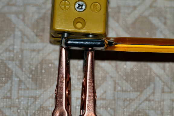
Figure 7
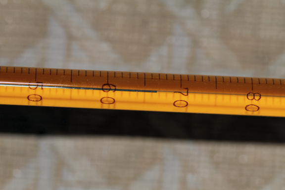
Figure 8
Now let’s
do this again but this time paying attention to CJC and seeing the
importance of CJC in the measurement. We will use the same setup as used in
Figure 6 but this time we will apply a reference junction temperature of 32
degrees F (0.0 C) as called out n the thermocouple reference tables. To
accommodate the cold junctions we will use a really simple and cheap ice
bath and the transition reference junctions shown in Figure 5. Those
familiar with this sort of measurement will be quick to point out the ice
bath should be in a Dewar’s (Vacuum) Flask and yes, the ice and water should
be distilled. For our learning purposes rest assured (I wouldn’t lie to you)
that a bucket of ice and Cleveland, Ohio USA tap water is just fine. There
are also various electronic ice point references out there, the Omega TRC
III comes to mind but we are not going to delve into them. The transition
reference junctions could also be easily made. I have some commercial
versions so I used them. Figure 9 represents our new and improved
measurement setup.
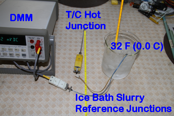
Figure 9
My ice bath
thermometer reads 32 degrees F (0.0 degrees C) and my hot junction
thermometer reads 65 degrees F (18.33 C). We exit our Type K thermocouple
using thermocouple alloys and go into the ice bath where copper alloy mates
with the T/C alloys at a temperature of 32 degrees F (0.0 degrees C) and
pass the signal along to our DMM. Let’s take a look at Figure 10.
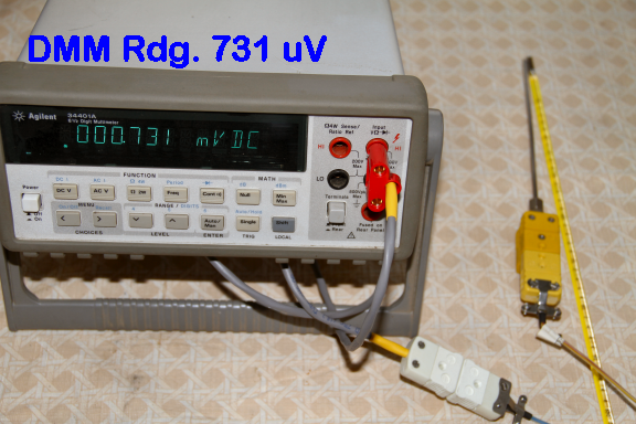
Figure 10
Earlier I mentioned the
precision thermometer measuring the T/C hot junction was reading 65 degrees
F (18.33 C). If I return to my Type K reference tables I see the milli-volt
output for 65 degrees F (18.33 C) should be 0.731 mV which is exactly what
we have. Go figure huh?
The results
of this little kitchen table experiment even surprised me. Considering my
ice point reference was nothing special and considering the allowable error
of the actual thermocouple I did not expect to get results within one degree
F. I submit this as proof that even a blind squirrel finds an occasional
acorn.
While pages
and pages of text can be written about CJC the objective here was to give
you the reader a very basic overview of what CJC is and one method to apply
it. I believe we can see as demonstrated the importance of CJC and how it
applies to the measurement plane. It is not as simple as measuring a T/C
output using a DMM to measure temperature. We will see more about CJC as we
continue but for now we will take a look at Thermocouple Accuracy or
Uncertainty.
Thermocouple Accuracy &
Specifications:
Before we
even begin to look at just how good a T/C measurement can be I want to
clarify something. When it comes to the measurement plane I see accuracy as
a qualitive term that denotes a degree of quality, I see error as a
quantative term which may be expressed numerically. I cringe when I hear
someone say the accuracy of an instrument is +/- 1% of reading or full
scale. That tells me the instrument is only 1% accurate with an allowable
error of 99%. That said, we will move along to
the accepted allowable uncertainties of thermocouples. Let’s also look at
some general T/C specifications. We will look at T/C types J, K and T.
Type J:
MAXIMUM TEMPERATURE RANGE
Thermocouple Grade
32 to 1382°F
0 to 750°C
Extension Grade
32 to 392°F
0 to 200°C
LIMITS OF ERROR
(Whichever is greater)
Standard: 2.2°C or 0.75%
Special: 1.1°C or 0.4%
COMMENTS, BARE WIRE ENVIRONMENT:
Reducing, Vacuum, Inert; Limited Use in
Oxidizing at High Temperatures;
Not Recommended for Low Temperatures
TEMPERATURE IN DEGREES °C
REFERENCE JUNCTION AT 0°C
Type K:
MAXIMUM TEMPERATURE RANGE
Thermocouple Grade
– 328 to 2282°F
– 200 to 1250°C
Extension Grade
32 to 392°F
0 to 200°C
LIMITS OF ERROR
(Whichever is greater)
Standard: 2.2°C or 0.75%
Above 0°C
2.2°C or 2.0% Below 0°C
Special: 1.1°C or 0.4%
COMMENTS, BARE WIRE ENVIRONMENT:
Clean Oxidizing and Inert; Limited Use in
Vacuum or Reducing; Wide Temperature
Range; Most Popular Calibration
TEMPERATURE IN DEGREES °F
REFERENCE JUNCTION AT 32°F
Type T:
MAXIMUM TEMPERATURE RANGE
Thermocouple Grade
– 328 to 662°F
– 200 to 350°C
Extension Grade
– 76 to 212°F
– 60 to 100°C
LIMITS OF ERROR
(Whichever is greater)
Standard: 1.0°C or 0.75%
Above 0°C
1.0°C or 1.5% Below 0°C
Special: 0.5°C or 0.4%
COMMENTS, BARE WIRE ENVIRONMENT:
Mild Oxidizing, Reducing Vacuum or Inert; Good
Where Moisture Is Present; Low Temperature
and
Cryogenic Applications
TEMPERATURE IN DEGREES °C
REFERENCE JUNCTION AT 0°C
All thermocouples support data like this
and this data plays a pivotal roll in thermocouple selection for a given
application. Beginning with the Maximum Temperature Range we see over what
range of temperatures which thermocouples are suited. Actual thermocouple
wire comes in several different grades which define the quality of the
actual wire. Thermocouple Grade wire is what the
name implies. The wire is manufactured to meet standard limits of error for
the T/C type. Special limits wire is a higher purity grade of wire with, as
can be seen, closer limits of error. Extension grade is just wire used
between a thermocouple and the instrument reading the thermocouple.
Pay attention
to the limits of error. Without special calibration what you see is what you
get. People frequently will state they wish to use a Type K thermocouple and
achieve an uncertainty of +/- 0.1 degree F or C. This is unrealistic as a
change of 0.1 degree C amounts to a change of about 4
uV in the thermocouple output. When
choosing a thermocouple for an intended application we need the thermocouple
to meet or exceed our range and uncertainty requirements.
When we see a
reference to Bare Wire this means the base alloy thermocouple with the
junction exposed to the atmosphere the thermocouple is used in. For example
a Type J thermocouple is made from Iron and Constantan alloy. A bare wire
Type J thermocouple would not be a good choice in a moist environment as the
iron would be prone to rust and corrosion. This would only be true when the
actual thermocouple alloy is exposed or bare. There is likely no limit to
the number of ways thermocouples can be constructed.
Making
A Thermocouple:
Since we
know a thermocouple is a junction of two dissimilar alloys if we have some
thermocouple wire we can build a thermocouple at the kitchen table. We will
start with a few lengths of bare Type K thermocouple wire.
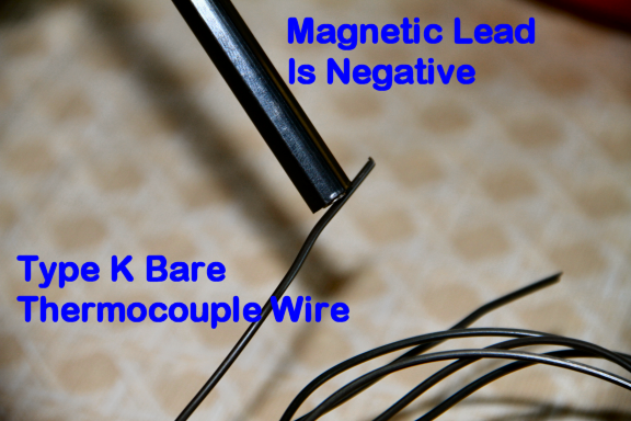
Figure 11
Worth noting is when using Type K T/C wire the Negative lead is
magnetic. This is useful as both alloys look the same, also worth noting is
in the case of a Type J T/C the Positive lead is magnetic. The wire used
here is AWG 12 (2.05 mm) which is pretty thick stuff but this thermocouple
would be suitable for use in a 2,000 degree F (1093 C) furnace application.
That is assuming it actually works.
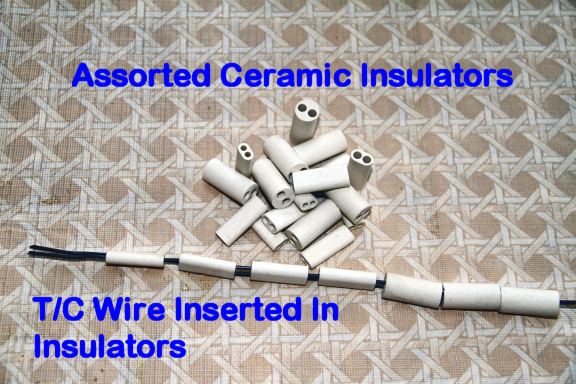
Figure 12
Figure 12 shows how we can
insert our T/C wire into several ceramic insulators. Insulators of this type
come in a wide variety of sizes and shapes. Several were used in Figure 12
as an example.
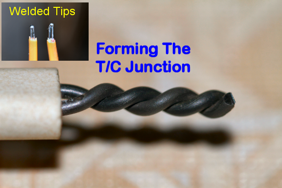
Figure 13
Figure 13 illustrates how
the actual junction of the dissimilar alloys is formed. I created a small
inset to the image showing some welded tips on AWG 22 thermocouple wire.
Thus far my very patient wife has been very good about my use of what is
“her” kitchen table. I feel it would be unwise to wander out to the backyard
shed and drag the Oxy / Acetylene welding outfit into her kitchen to weld
the tip of the junction on our new thermocouple. However, I should point out
that it is very, very important when welding T/C tips that only enough heat
be used to weld the tip and only at the tip. Excessive heat and heat not
applied correctly will alter the composition of the alloys creating a bad
and inaccurate thermocouple. I cannot stress enough the importance of this
step, especially when working with lighter gauge T/C wire.
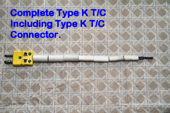
Figure 14
Figure 14 illustrates our finished product. A standard
thermocouple connector has been added. While not very pretty our
thermocouple should be functional, remember it is only an example. This
thermocouple could be inserted into for example a ceramic protection tube or
alloy protection tube. The next logical step would be to test our newly made
thermocouple. I guess I should come up with a way we can see if this thing
actually works. The classic statement applies at this point in that “it
looks good on paper”.
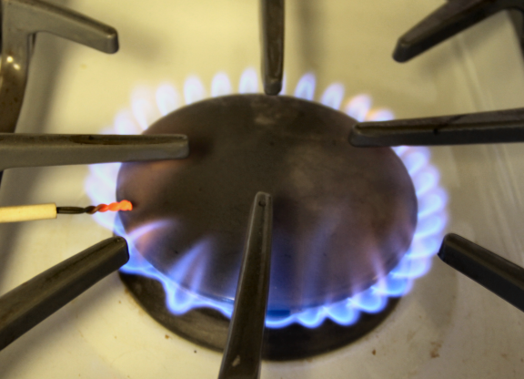
Figure 15
I have been informed by my
most patient wife that if anything goes wrong with using “her” stove this
will be my first and last blog. It could also mark the end of my life as I
know it. Figure 15 illustrates our new home manufactured thermocouple at the
kitchen table. The burner natural gas heat has our thermocouple radiating a
nice orange color so we can assume it is pretty hot at the tip junction.
Using some Type K thermocouple extension wire and a mating plug for our
thermocouple I have connected the thermocouple to an instrument suited for
measuring thermocouple output. Let’s take a look at thermocouple temperature
at the junction and see what we have here.
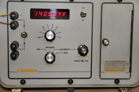
Figure 16
The device pictured in Figure 16 is an old but accurate and reliable
Omega manufacture Omni-Cal used in the testing and calibration of
thermocouples. This same instrument was marketed under several brand names
about 20 years ago. Every now and then I drag it into work and check the
calibration of it. For an instrument over 20 years old it still maintains
very good accuracy and I occasionally replace the battery NiCad pack. The
instrument is setup to measure a signal from the A input from a Type K
thermocouple and display the temperature in Degrees F. We can see our
thermocouple is reading a temperature of 1,408.4 degrees F. (764.67 C).
Prior to heating the thermocouple I did compare it to a precision mercury
glass thermometer at room temperature and it was perfect. Instruments like
this take into consideration the CJC we already discussed as does all modern
temperature indicating and measuring instruments.
Note the
connection point where the T/C extension wire mates with the instrument’s
connectors. Generally speaking when using thermocouple extension wire,
designed for low temperature environments, the red colored lead is the
negative. For example Type K is Red and Yellow, Type J is Red and White and
Type T is Red and Blue. In each case the Red lead is the T/C negative
output. I constantly see people new to the thermocouple world insist on
making the Red lead the Positive signal lead. Weird things happen when this
error is made.
Thermocouple Signal
Conditioning:
I like to
define “signal conditioning” as taking the signal you have and converting it
to the signal you want. We know a thermocouple outputs a small milli-volt
signal proportional to temperature, we know it is a non linear signal and we
know the thermocouple reference table’s reference to 32 degrees F (0.0 C).
One very
simple and yet very accurate means of conditioning the low milli-volt signal
from a thermocouple to something useable is a small device known as a
“Temperature Transmitter” a few images of which are shown in Figure 17.
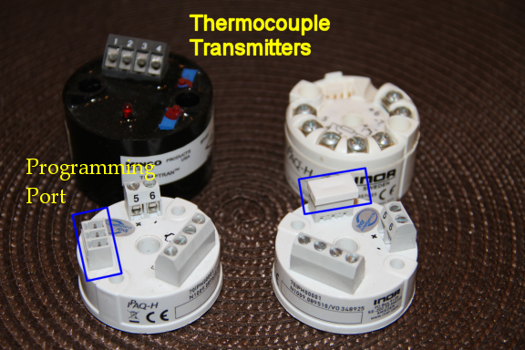
Figure 17
These small devices available from a wide range of manufacturers can
take an input directly form a thermocouple and output signals like 0 to 20
mA, 4 to 20 mA, 0 to
5 volts, 0 to 10 volts as well as other outputs for a given temperature
range. The black device (upper left) was manufactured by Minco Manufacturing
or actually marketed by them and is about 20 plus years old. Units like this
were designed for a specific temperature range and output as well as
thermocouple type. Newer units offer programming options as to input, output
as well as working with mV inputs for example from strain gauges. These
devices also take care of all the linearization curves we looked at earlier
providing a nice clean linear output.